
Zone maps, or “queries go brrr”
Waiting sucks. Let's use zone maps to move fast and read less.


Waiting sucks, whether you're a trader eager for so-called “real-time” insights or a patient awaiting test results. In either case, a data system might be the bottleneck, waiting for records to stream in from storage. Zone maps reduce that delay by skipping irrelevant records. Each “zone” stores summary statistics (such as a minimum and maximum), so that the data system can skip reading records that fail to meet the query criteria. In this post, we’ll look at why zone maps matter and how they’re implemented in Vortex and Parquet.
A Simple Example of Min/Max Zone Maps
Zone maps record summary statistics about a specific region of a dataset. Typically, a “zone” is a contiguous set of records in a dataset. The simplest and most common kind of statistics used in a zone map are the minimum and maximum value of a particular column in that sequence of rows.
Consider, for example, a few rows from the familiar Iris dataset:
| Row | Sepal length | Sepal width | Petal length | Petal width | Species |
|---|---|---|---|---|---|
| 1 | 5.1 | 3.5 | 1.4 | 0.2 | I. setosa |
| 2 | 4.9 | 3.0 | 1.4 | 0.2 | I. setosa |
| 3 | 4.7 | 3.2 | 1.3 | 0.2 | I. setosa |
| 4 | 4.6 | 3.1 | 1.5 | 0.2 | I. setosa |
| 5 | 5.0 | 3.6 | 1.4 | 0.3 | I. setosa |
| 6 | 7.0 | 3.2 | 4.7 | 1.4 | I. versicolor |
| 7 | 6.4 | 3.2 | 4.5 | 1.5 | I. versicolor |
| 8 | 6.9 | 3.1 | 4.9 | 1.5 | I. versicolor |
| 9 | 5.5 | 2.3 | 4.0 | 1.3 | I. versicolor |
| 10 | 6.5 | 2.8 | 4.6 | 1.5 | I. versicolor |
| 11 | 5.7 | 2.8 | 4.1 | 1.3 | I. versicolor |
| 12 | 6.3 | 3.3 | 6.0 | 2.5 | I. virginica |
| 13 | 5.8 | 2.7 | 5.1 | 1.9 | I. virginica |
| 14 | 7.1 | 3.0 | 5.9 | 2.1 | I. virginica |
| 15 | 6.3 | 2.9 | 5.6 | 1.8 | I. virginica |
| 16 | 6.5 | 3.0 | 5.8 | 2.2 | I. virginica |
The following is one possible zone map with five zones. Each zone stores a minima and maxima for three of the five columns.
| Zone | Rows | Sepal length | Petal length | Petal width |
|---|---|---|---|---|
| 1 | 1-3 | [4.9, 5.1] | [1.3, 1.4] | [0.2, 0.2] |
| 2 | 4-6 | [4.6, 7.0] | [1.4, 4.7] | [0.2, 1.4] |
| 3 | 7-10 | [5.5, 6.9] | [4.0, 4.9] | [1.3, 1.5] |
| 4 | 11-13 | [5.7, 6.3] | [4.1, 6.0] | [1.3, 2.5] |
| 5 | 14-16 | [6.3, 7.1] | [5.6, 5.9] | [1.8, 2.2] |
Suppose we must evaluate this SQL query:
SELECT * from tbl WHERE "Petal width" < 1.0
Using only the zone map, we may conclude that every row from seven onward fails the WHERE clause because their petal widths are at least 1.3. We need not even load those last three zones from storage! We also know that every row in the first zone passes the WHERE clause and we know at least one row in the second zone passes.
This zone map allowed us to skip reading three out of five zones. Those zones comprise 5/8ths of the data. If bandwidth was our only bottleneck, our query might run over twice as fast!
However, not every query can leverage a zone map, for example, this query must scan our entire dataset:
SELECT * FROM tbl WHERE "Petal width" < 1.9
Moreover, not every column is suited to a zone map! Consider the following query which searches for samples with a small but reasonable range of Sepal length.
SELECT * FROM tbl where "Sepal length" >= 6.0 AND "Sepal length" <= 6.2
Although no samples match this WHERE clause, our metadata table only allows us to eliminate zone 1 and zone 5 whose sepal length values are respectively fully below 6.0 or fully above 6.2.
The issue with the sepal length column is that it does not cluster with the ordering of the rows. In the context of zone maps, a numeric column is said to cluster when values from nearby rows are nearby on the number line. The petal width column demonstrates clustering. In particular, the rows of the Iris data happen to be ordered by their species which are, famously, fairly well distinguished by petal width and not so well distinguished by sepal length.
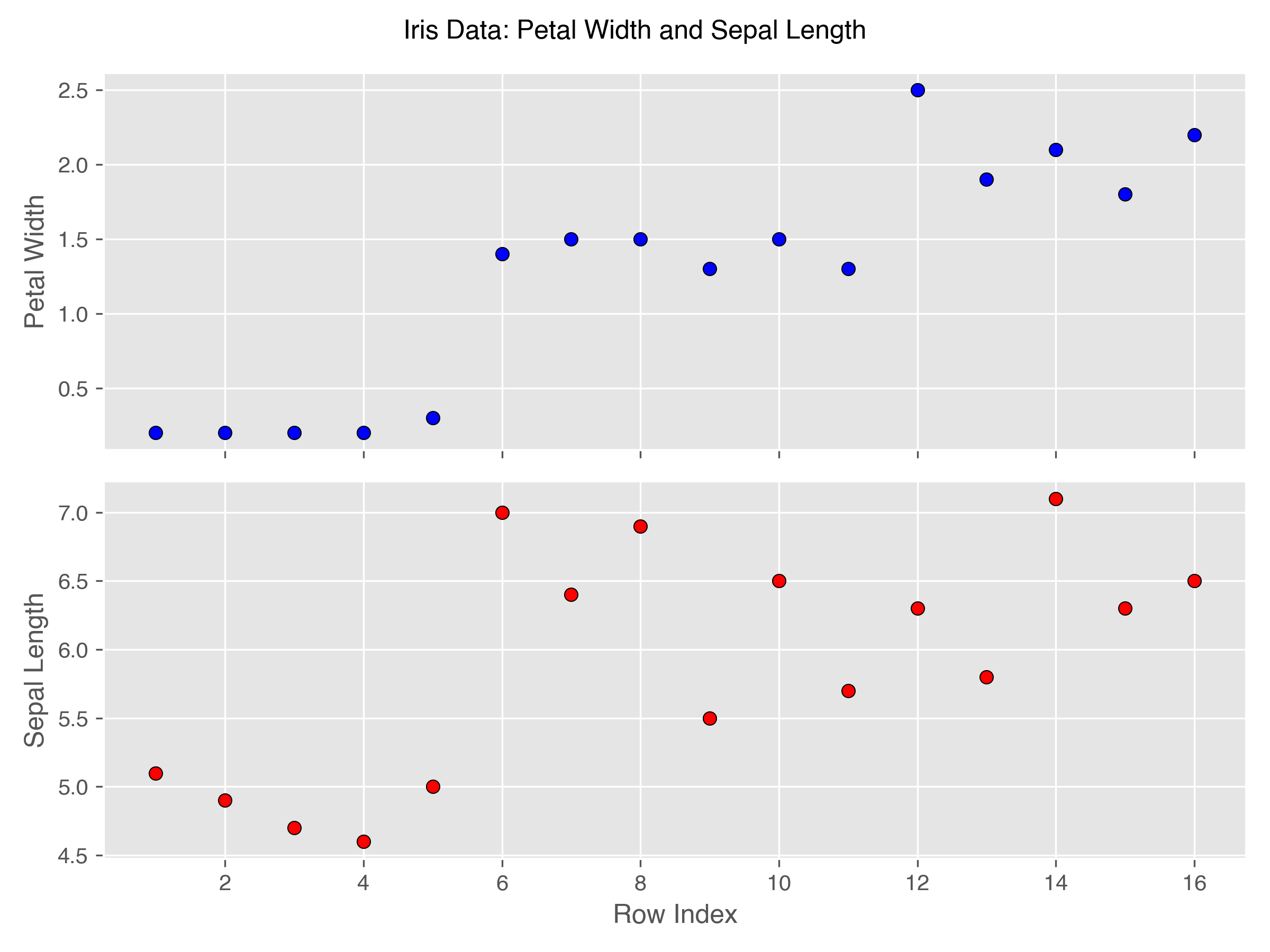
In the top sub-figure, notice that points with similar row indices, tend to have similar y-coordinates. In contrast, in the bottom sub-figure, the range of y-coordinates is much larger, particularly after row five.
Timestamps are perhaps the most common example of a clustered column because logs are inserted roughly in timestamp-order. Order numbers can be a clustered column. In genetics & genomics, the gene and the genetic locus are often clustered columns.
Beyond Min/Max: Bloom Filters
While zone maps of minima and maxima are common, a zone map may store any kind of metadata that helps a query system to avoid reading data. For example, the count of null rows can accelerate IS (NOT) NULL queries. Some formats, such as Apache Parquet and ORC, store bloom filters, a kind of approximate membership query (AMQ) data structure. There are many good descriptions of Bloom filters, such as this one, so we won’t cover them again here; however, an AMQ data structure, such as a Bloom filter, can help where a minimum and maximum is too coarse.
Consider for example, a column of UUIDs. By design, a UUID column will not cluster because it is meant to be uniformly distributed. Instead, the minima and maxima will grow further and further apart as the zone grows in size. Such a zone map is of limited utility because very few values are not contained within that range.
Bloom filters are a solution to this problem. As long as a single zone has relatively few distinct values, the Bloom filter will compactly—albeit imprecisely—represent those distinct values. Equality and IN queries can instead query the Bloom filter and avoid reading any zone which the Bloom filter knows does not contain matching records.
Geospatial Metadata
We currently lack the expertise to describe it well, but there are even more exotic metadata in use in production. For example, authors from Google have described the use of geospatial metadata to accelerate queries about distances on the surface of Earth (see Section 5.3.10 of Edara & Pasumansky “Big Metadata” and Google’s S2 Geometry library). In general, any small summary that helps skip data can be included in a zone map.
Concrete Implementations
As far as this author can tell, the earliest discussion of zone maps was Moerkotte’s 1998 paper “Small Materialized Aggregates”. Since then, many systems have implemented them under a variety of names: ClickHouse “Data Skipping Indices”, Monet DB “correlated orderings”, IBM Netezza & Oracle “zone maps”, Postgres “Block Range Indices”, Parquet “page indices”, ORC “indexes”, Snowflake “micro-partitions”, Vertica “ROS containers”, and Google Capacitor’s “range constraints”, to name just eleven of the countless implementations.
Implementations also vary widely in how they size a zone: Oracle storage indices use 1 MB zones, Postgres blocks and Parquet pages are usually 8 KB, ORC stripes are 64 MiB and their row groups are 10,000 rows.
The Design and Implementation of Zone Maps
We recently implemented zone maps for Vortex, our new columnar file format. In preparation for doing so, we reviewed the extensive literature around zone maps and assessed how modern databases and hardware interact with the conclusions of that body of literature. Two major design goals crystalized for us:
- Reading a zone map from storage must not require any copies or deserializations.
- Zone maps need not be tied to physical blocks, thanks to slice-able lightweight compression.
The first goal is a bit old hat at this point. MessagePack, Cap’n Proto, Arrow, and FlatBuffers all emerged in the early twenty-teens, championing minimal-overhead data access: no decompression, no pointer swizzling. Modern storage systems are relatively high-bandwidth, so we can trade a big storage footprint for less CPU overhead. This is even more true for zone maps which lie on the critical path towards retrieving the data.
As for the second goal, zone maps of the last two decades were often used with block compression pages. The best compression ratio is achieved when the compressor has access to the most data, ideally the whole column. However, compressing the whole column into one page means reading any one row requires decompressing every row. Most formats expose a page size parameter and ask the user to choose a size that balances compression ratio against random access overhead.
Lightweight compression schemes like FSST, FastLanes, and ALP break this tension by delivering compression ratios competitive with block compressors (e.g. Zstd, Snappy) without compromising constant-time access to any one row. This allows us to tune the I/O block size to the physical characteristics of the underlying storage system while separately tuning the zone size to the logical characteristics of the data. We could choose the same zone size for every column to allow pruning one column by a predicate evaluated on the zone map of a different column. We could also choose variable and data-dependent zone sizes that minimize zone map size while maximizing the effectiveness of our metadata.
Zone maps in Vortex
Zone maps are stored in the footer of a Vortex file. In the best case, the initial read, which retrieves the file layout description, also includes the zone maps. Once read, no deserialization is necessary because Vortex pervasively uses zero-copy representations of both metadata and data.

By default, zones are blocks of 8,192 rows. As we mentioned above, zone blocks need not be aligned to compression block size which are instead tuned to the page size of the underlying storage system. A consequence of this decoupling is that zones and compression blocks arbitrarily overlap with one another. In columns with large values, such as column of images, a single zone might contain several compression blocks. A single block might even contain rows from two different zones. The situation is reversed for a 32-bit integer column where each block may contain tens of zones. In either case, our lightweight cascading compression allows efficient slicing, enabling us to read a row range without paying the cost of full decompression.
Zone Maps in Parquet
Until 2017, Parquet’s zone maps were scattered around the file, requiring multiple reads to load them and then Thrift deserializations to access them. The Parquet community knew this was a problem and addressed this issue by adding page indices to the spec. For each row group and column, all the page minima and maxima are stored together in the footer. This substantially improved upon the scattered situation, allowing the zone map for a column chunk to be read and deserialized as one object. Over time, the major Parquet implementations added support:
- 2018: The Parquet Java library added support first.
- 2021: Spark added support in 3.2.0.
- 2022: DataFusion added support in 14.0.0.
- 2023: The Parquet C++ library added support in Apache Arrow 12.0.0.
Six years later, the Parquet ecosystem has functional zone maps, but they remain entangled with physical structures in Parquet. Both pages and the row groups that contain them are chosen to meet byte-size targets. This is reasonable given that Parquet relies on block compression to achieve small file sizes.
Future Work
Dear reader, with what kinds of data do you work? Are there domain-relevant statistics that may accelerate queries against your data? Maybe a clever transformation like Google’s S2 cells or an approximate quantiles sketch? Share your insight with us in an issue and maybe contribute directly to the project!
Follow along with us as we develop a well-specified and backwards compatible file format and build out an extensive library for working with compressed arrays in-memory, on-disk, and over-the-wire. Star the Vortex GitHub repository and peruse the documentation, where you will find descriptions of the high-level concepts, the file format, and our integrations with the Python data science ecosystem.
Finally, subscribe to an email newsletter of this blog for a steady stream of both engineering practicalities as well as research digests on the design and implementation of column-oriented storage.
Annotated Bibliography
- Moerkotte, Guido. “Materialized Aggregates: A Light Weight Index Structure for Data Warehousing”. VLDB 1998. https://www.vldb.org/conf/1998/p476.pdf.
- Zukowski, Martin et al. “Cooperative Scans: Dynamic Bandwidth Sharing in a DBMS”. VLDB 2007. https://15721.courses.cs.cmu.edu/spring2016/papers/p723-zukowski.pdf.
- Herrera, Alvaro. “[RFC] Minmax indexes”. Post to pgsql-hackers@postgresql.org. 2013-06-14. https://www.postgresql.org/message-id/20130614222805.GZ5491@eldon.alvh.no-ip.org.
- Budalakoti, Suratna et al. “Automated Clustering Recommendation With Database Zone Maps”. SIGMOD 2024. https://dl.acm.org/doi/pdf/10.1145/3626246.3653397
In this paper, Oracle describes an algorithm for selecting a set of columns on which to create zone maps in order to reduce the number of zones accessed by a set of queries.
- Schulze, Robert, et al. “ClickHouse - Lightning Fast Analytics for Everyone”. VLDB 2024. https://www.vldb.org/pvldb/vol17/p3731-schulze.pdf.
Section 3.2 discusses ClickHouse’s zone maps, which are called “skipping indices”. They support three kinds of metadata: min-max, finite set, and bloom filters.
- Edara, Pavan & Pasumansky, Mosha. “Big Metadata: When Metadata is Big Data”. VLDB 2021. https://www.vldb.org/pvldb/vol14/p3083-edara.pdf
This is a fantastic paper. Section 4 describes how to work with zone maps weighing tens of terabytes. Section 5 describes, in depth, how to transform SQL predicates into predicates on zone maps that enable pruning of zones without matching rows. Sub-sub-section 5.3.10 describes the use of geospatial indices to prune queries which filter on intersecting geographies.
- Melnik, Sergey, et al. “Dremel: A Decade of Interactive SQL Analysis at Web Scale” VLDB 2020. https://www.vldb.org/pvldb/vol13/p3461-melnik.pdf.
Section 6.1 describes Google’s Capacitor library which collects various smart data access techniques into a common library used by many of Google’s data systems including F1, MapReduce, and BigQuery. Capacitor provides, in the data access layer, zone map based pruning.
- Ziauddin, Mohamed, et al. "Dimensions Based Data Clustering and Zone Maps”. VLDB 2017. https://vldb.org/pvldb/vol10/p1622-ziauddin.pdf.
- Boncz, Peter, et al. “FSST: Fast Random Access String Compression” VLDB 2020. https://www.vldb.org/pvldb/vol13/p2649-boncz.pdf.
- Afroozeh, Azim, et al. “The FastLanes Compression Layout: Decoding >100 Billion Integers per Second with Scalar Code”. VLDB 2023. https://www.vldb.org/pvldb/vol16/p2132-afroozeh.pdf.
- Afroozeh, Azim, et al. “ALP: Adaptive Lossless floating-Point Compression”. SIGMOD 2023. https://dl.acm.org/doi/pdf/10.1145/3626717.


